

Differentiable Physics: Teaching Simulators to Think (and Feel Derivatives)
A beginner's guide to differentiable physics simulators
Let’s say you’re trying to teach a robot to pour coffee.
You run a simulation — and instead of pouring into the mug, it confidently dumps hot virtual espresso onto the table. Not ideal.
With a normal simulator, you’d shrug, tweak some parameters, hit run again, and hope for the best.
In a differentiable simulator, though, something magical happens: the simulator tells you exactly how to tweak those parameters to make the pour better next time.
Welcome to the world of differentiable physics — where simulations don’t just predict the future, they learn from it.
So What Even Is Differentiable Physics?
At its core, a normal physics simulator answers questions like:
“Given a mug of coffee, some gravity, and a bad pouring action, where will the coffee land?”
It’s a one-way street: you give it inputs (forces, parameters, states), and it gives you outputs (positions, velocities, energy, etc.).
But if you then ask,
“How should I change the pouring action to make the coffee land in the cup instead?”
the simulator just stares at you blankly. It doesn’t do “why”.
Differentiable physics fixes that by making the simulator mathematically transparent — it not only runs the physics forward but also tells you how sensitive the results are to each input. In other words, it gives you gradients.
So instead of just knowing what happened, you know how to make it happen better next time.
A Bit of Math Without the Trauma
A normal simulator computes:
$$x_{t+1} = f(x_t, u_t, p)$$
where \(x_t\) is your system’s state (like position and velocity) at time $t$, \(u_t\) is control input (like motor torque), and $p$ are physical parameters (like mass, gravity and viscosity).
A differentiable simulator also gives you:
$$\frac{\partial x_{t+1}}{\partial u_t}, \quad \frac{\partial x_{t+1}}{\partial p}$$
That fancy notation basically means:
“If I nudge this parameter by a smidge, how much does the outcome change?”
This means we can see how tiny changes in control or parameters affect the next state — the same idea that makes neural networks trainable via backpropagation. This is gold for optimization. Now, your simulator can be plugged straight into any standard gradient-based learning tools and the physics becomes trainable.
Why Gradients Change Everything

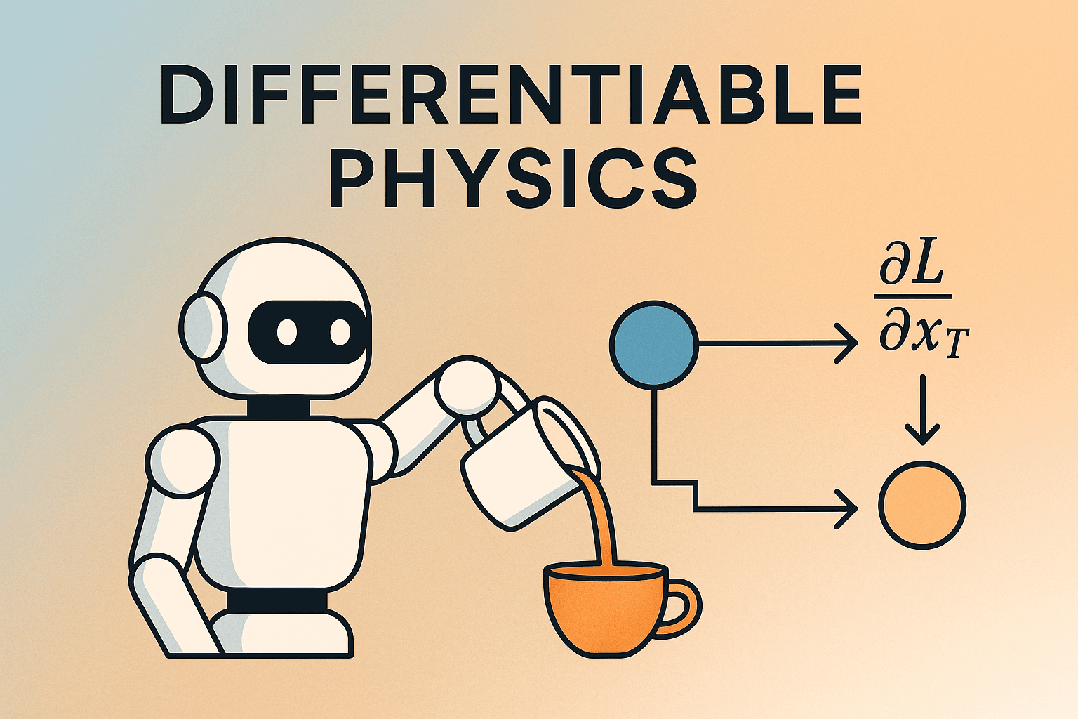
(Image: A simple visual explaining how differentiable physics works. The robot’s action $u$leads to a final state (\(x_T\)) — like pouring coffee into a cup — which produces a loss (𝐿) if the outcome isn’t perfect. Gradients (\(\nabla_{u} L\)) flow backward, telling the simulator how to adjust the action to improve the next pour, such that the loss reduces.)
The beauty of differentiable physics lies in optimisation.
Say you have a loss function (a measure of how well the robot poured the coffee):
$$L = \| x_T - x^* \|^2$$
where \(x_T\) is the final simulated state, and \(x^*\) is your goal (like a mug full of coffee poured by your robot).
With differentiable physics, you can compute:
$$\nabla_{u} L = \frac{\partial L}{\partial x_T} \frac{\partial x_T}{\partial u}$$
which in simple terms says something like, “If you’d tilted the cup this much more, you’d have been this much closer to perfect”. You can use this to directly adjust your control inputs $u$ using gradient descent — just like training a neural network.
That’s the magic of differentiable physics — it turns physical cause and effect into gradients that machines can learn from. No black-box reinforcement learning, no random trials. The simulator itself becomes a learning machine.
Under the Hood: Differentiating Through Physics
Okay, so you might be wondering — how do you actually take derivatives of something as messy as a physics simulator? It’s not like you can just open a textbook and find a neat formula for “∂coffee/∂tilt-speed”.
No, it’s a bit trickier. Physical simulations involve:
Discontinuities (like collisions or contact)
Integrators (like Euler or Runge-Kutta)
Constraints (like joints or limits)
All of which are less than helpful in making things differentiable. The secret lies in making every step of the simulation play nicely with gradients.
Step 1: Make the Simulator Smooth(-ish)
Real-world physics can be messy. Think about pouring coffee — if your mug hits the table, it’s an instant, sharp collision. Mathematically, that’s what we call a discontinuity — the motion goes from “moving” to “stopped” in no time. Gradients, which measure how smoothly things change, hate that kind of drama.
So differentiable simulators try to smooth out those rough edges a little:
Instead of saying “the mug hits the table at exactly this instant,” they use a soft contact model, as if the mug and table have a tiny cushion of air. The mug gently squishes in, making the transition continuous.
Friction — normally a harsh stick-then-slide behavior — is modeled as a smooth curve.
That way, when you ask “how would a slightly softer pour or different tilt change the splash height?” the math stays calm — no infinities, no meltdowns, just gradients that flow nicely.
Step 2: Use Integrators That Play Nice with Gradients
Most physics engines update motion step-by-step with integrators like Euler or Runge–Kutta.
A differentiable simulator, though, does better: it can efficiently compute how each state depends on the previous one. It’s like being able to know how every small change in wrist angle, mug tilt, or pour rate affects the final coffee level.
So instead of just computing:
$$x_{t+1} = f(x_t, u_t)$$
they can quietly compute and record how sensitive \(x_{t+1} \) is to every variable.
When you hit “backpropagate,” those sensitivities (the “Jacobians”) chain together backwards in time — like unrolling the tape of the simulation. (“If I had poured just a little slower here, I’d have hit the perfect amount.”)
Step 3: Let Automatic Differentiation Do the Heavy Lifting
Thanks to frameworks like JAX or Taichi, you don’t have to do calculus by hand.
Every operation — addition, multiplication, even matrix math — automatically keeps track of its derivative.
So when you say “simulate 100 time steps and minimize the spill,” the system quietly builds a computational graph of everything that happened.
Then, when you call .backward() or .grad(), the gradients flow through that graph like magic.
It’s physics, but with built-in self-reflection.
Putting It All Together
At the end of the day, “differentiating through physics” just means "letting your simulator understand how its outputs depend on its inputs”.
So when your robot pours coffee too fast, the simulator doesn’t just say “oops, that spilled” — it also says “if you’d tilted 5° less, you’d have nailed it.”
That’s the power of gradients flowing through time, through equations, and through your robot’s tiny virtual neurons.
When Physics Meets AI
For years, physics and AI were like two geniuses at opposite ends of the classroom — one obsessed with equations, the other with data. Both brilliant, both a little smug, and both pretending the other didn’t exist.Now, thanks to differentiable physics, they’re finally collaborating — and it turns out they make a really good team.
Applications Beyond Coffee
Differentiable physics isn’t just about robotic baristas. It’s reshaping how we approach any problem involving physics and optimisation.
Robots that learn faster: Instead of brute-forcing policies through endless reinforcement learning trials (robot pouring coffee all over your simulated coffee table), you can differentiate through the simulation. That gives you a direct signal for how to improve control — no random trial-and-error needed.
Easier system identification: Got a simulation where the robot doesn’t quite behave like in the real world? Just let the gradients flow. The simulator can automatically tweak its parameters (like joint damping or motor lag) until it matches reality. It’s like the simulator saying, “Oh, my bad — I thought we were on the moon. Let’s adjust the gravity parameter.”
Aiding Robot Design: Want to design a soft robot that slithers gracefully like an eel? Or a structure that folds into a flower when heated? You can specify your goal and let the simulator backpropagate through physics to find the perfect design. Welcome to the age of inverse design.
Differentiable physics opens the door to accelerate research and improve tools in other fields as well, such as graphics and animation (inverse design for realistic physical effects, adjust material motions to match reality, etc.), and material & fluid sciences (optimise material structures, fluid flows, molecular configurations etc.).
When physics meets AI, we move from modeling the world to optimising it. Differentiable physics blurs the line between simulation and learning. Instead of treating simulators as “truth machines” that tell us what happens, we can now teach them what we want to happen.
This opens up an era of end-to-end trainable physics systems, where:
Neural networks predict control inputs.
Simulators propagate both states and gradients.
The whole loop optimises itself.
It’s not just “simulate and observe” anymore — it’s: “Simulate, differentiate, and improve.”
Everywhere there’s a physical process — from how a robot walks, to how a drone flies, to how your robot pours coffee — gradients can make it smarter, faster, and more efficient. We’re basically giving simulations a sixth sense — the sense of how to improve, and this is a game-changer. Instead of fumbling around for millions of tries like a toddler learning to walk, a robot can use gradient feedback to master a task in just a few hundred runs.
Take Google’s Brax simulator, for instance: it uses differentiable physics on TPU clusters to train walking, running, and jumping robots thousands of times faster than traditional RL. Or MIT’s DiffTaichi, which simulates elastic objects “188x faster than TensorFlow implementations” — making it possible for neural controllers to optimise in mere tens of iterations.
What’s next?
As this field matures, we will see more simulators that don’t just describe — they help build.
Imagine simulators that jointly optimize a robot’s shape, materials, and control system. Or digital twins that continuously fine-tune themselves based on sensor data.
VFX artists and game designers might use self-learning physics engines to automatically match animation physics to real footage. Engineers could design, test, and perfect structures — all before a single bolt is turned in real life.
In short, differentiable physics can turn simulation from a descriptive tool into a creative collaborator — a kind of physics buddy that not only explains reality but also helps improve it.
Tools of the Trade
If you’re curious about differentiable physics but don’t want to wrestle with equations, you’re in luck — there are several open-source frameworks that handle the heavy math for you while still letting you play with real simulations:
DiffTaichi – Super fast, highly expressive, and written by people who clearly love math.
Brax – Google’s JAX-based simulator for reinforcement learning with physics gradients baked in.
Tiny Differentiable Simulator (TDS) – The name says it all: small, elegant, and surprisingly powerful.
Nimble Physics – Great for robotics, built to play nicely with neural nets.
DiffSim, DiffCloth – For when you want your simulations to flow, bend, or squish — literally.
Newton - A clean, modular differentiable physics framework with a strong focus on usability and integration with deep learning workflows.
Each of these frameworks gives you a taste of differentiable physics without needing a PhD in calculus — just curiosity and a bit of code.
Further Reading
A Review of Differentiable Simulators (Newbury et al., 2024) - a very accessible and comprehensive survey paper on differentiable simulators.
“Introduction to Differentiable Physics” (Physics-Based Deep Learning) - for a more technical understanding of the topic with practical example.